Scientific work is visual. A researcher does not only ask an AI co-scientist for prose or code. They ask it to draw a cell, sketch an orbital transfer, explain a circuit, turn a mechanism into a figure, and revise that figure until it is clear enough to put in a report. That is why image models matter inside K-Dense Web, K-Dense BYOK, and Scientific Agent Skills. They are not a decorative layer. They are part of the research loop.
We wanted to know how the newest fast image model we have been testing, Nano Banana 2 Lite, behaves on scientific figures. Speed is obviously attractive, but scientific diagrams are a hard case for image generation because they demand accurate structure and legible text at the same time. A pretty but mislabeled figure is worse than a slow figure, because it can teach the wrong thing with confidence.
So we ran a controlled benchmark. We generated 240 scientific figures: four image models, 20 prompts, and three samples per prompt. Every prompt was identical across models. Every image was scored blind against the original prompt on a five-part rubric. The result is a clean speed-quality frontier: Nano Banana 2 Lite is dramatically faster, while GPT Image 2 produces the strongest raw scientific figures.
The Short Version
The headline is that Nano Banana 2 Lite returns a 1K scientific figure in about 3.8 seconds median, compared with 49.0 seconds for GPT Image 2. That is roughly a 13x speedup. Across a real research session, where a figure is revised several times and a report may need dozens of visuals, that difference changes the experience from batch waiting to interactive iteration.
The quality story is different. GPT Image 2 had the highest raw composite quality score, 8.64 out of 10, and led every rubric dimension. Nano Banana 2 Lite scored 6.70 out of 10, with its weakest dimension being scientific accuracy. If the only goal is the best single figure and latency does not matter, GPT Image 2 is the quality winner.
Where Nano Banana 2 Lite wins is the combined operating point. Under the benchmark's explicit overall score, 70 percent quality and 30 percent speed, Nano Banana 2 Lite ranks first with an overall score of 76.9. That is not the same as saying it is the most accurate image model. It means its speed is large enough to change the product tradeoff when scientific figure generation is a repeated tool call inside an agentic workflow.
 Figure 1. Overall leaderboard. The overall score is 70 percent quality and 30 percent speed. Under that weighting,
 Nano Banana 2 Lite ranks first because its speed score is 100, even though GPT Image 2 leads raw quality.
What We Tested
The benchmark compared four image models: Nano Banana 2 Lite, Nano Banana 2, Nano Banana Pro, and GPT Image 2. Nano Banana 2, Nano Banana Pro, and GPT Image 2 were accessed through OpenRouter. Nano Banana 2 Lite was accessed through its current Google AI Studio API surface because K-Dense is participating in the model's Early Access Program. The generation settings targeted 1K, 16:9 figures where supported, and every model completed all 60 generations with zero errors.
The prompt set covered 20 scientific and engineering figures across 15 disciplines. The tasks included a eukaryotic animal cell diagram, the central dogma, Michaelis-Menten kinetics, a neuronal action potential, an SN2 mechanism, a titration curve, projectile motion, Young's double-slit experiment, a non-inverting op-amp, a stress-strain curve, a four-stroke engine cycle, a Rankine cycle, airfoil aerodynamics, a Hohmann transfer, an H-R diagram, a stellar life cycle, a black-hole anatomy diagram, plate tectonics, and a crystal-structure plus phase-diagram figure.
These were deliberately label-heavy prompts. They asked for titles, axes, equations, components, phases, leader lines, and domain-specific relationships. That matters because scientific image generation fails in two different ways. It can fail visually, producing cluttered or unreadable figures, and it can fail scientifically, producing a clean diagram that encodes the wrong relationship.
| Model | Provider | Model ID | Images | Median Latency |
|---|---|---|---|---|
Nano Banana 2 Lite |
Google AI Studio | instant-ramen |
60 | 3.8 s |
| Nano Banana 2 | OpenRouter | google/gemini-3.1-flash-image |
60 | 11.1 s |
| Nano Banana Pro | OpenRouter | google/gemini-3-pro-image |
60 | 19.2 s |
| GPT Image 2 | OpenRouter | openai/gpt-image-2 |
60 | 49.0 s |
The full run generated 240 images in about 9.3 minutes of wall-clock time with concurrency set to 10. The benchmark used up to three attempts for transient provider failures, but the final corpus was complete: 240 generated images and 240 scored images.
How We Scored Scientific Figures
Every image was scored by Claude Opus 4.8 as a blind vision judge. The judge saw the prompt and the image, but not the model identity. Scores were assigned on a 1 to 10 scale across five dimensions, and the final composite was computed in code from the weighted rubric rather than delegated to the judge as a single holistic opinion.
The weights intentionally favor the things that matter most in a scientific figure. Scientific accuracy carries 30 percent of the score, text legibility and correctness carries 25 percent, prompt adherence carries 20 percent, visual clarity carries 15 percent, and aesthetic quality carries 10 percent. In other words, a beautiful figure with wrong labels should not win.
| Dimension | Weight | What It Measures |
|---|---|---|
| Scientific Accuracy | 30% | Correct structures, relationships, processes, quantities, equations, and domain conventions |
| Text Legibility and Correctness | 25% | Whether labels, titles, equations, and units are sharp, present, and spelled correctly |
| Prompt Adherence and Completeness | 20% | Whether the figure includes the requested elements, not just a plausible subset |
| Visual Clarity and Organization | 15% | Whether the composition is readable, well organized, and unambiguous |
| Aesthetic and Professional Quality | 10% | Whether the figure looks polished enough for a professional scientific context |
This rubric is strict by design. The benchmark is not asking which model makes the prettiest image in a general sense. It is asking which model makes figures a scientist could actually use, critique, and revise inside a research workflow.
Speed Changes the Research Loop
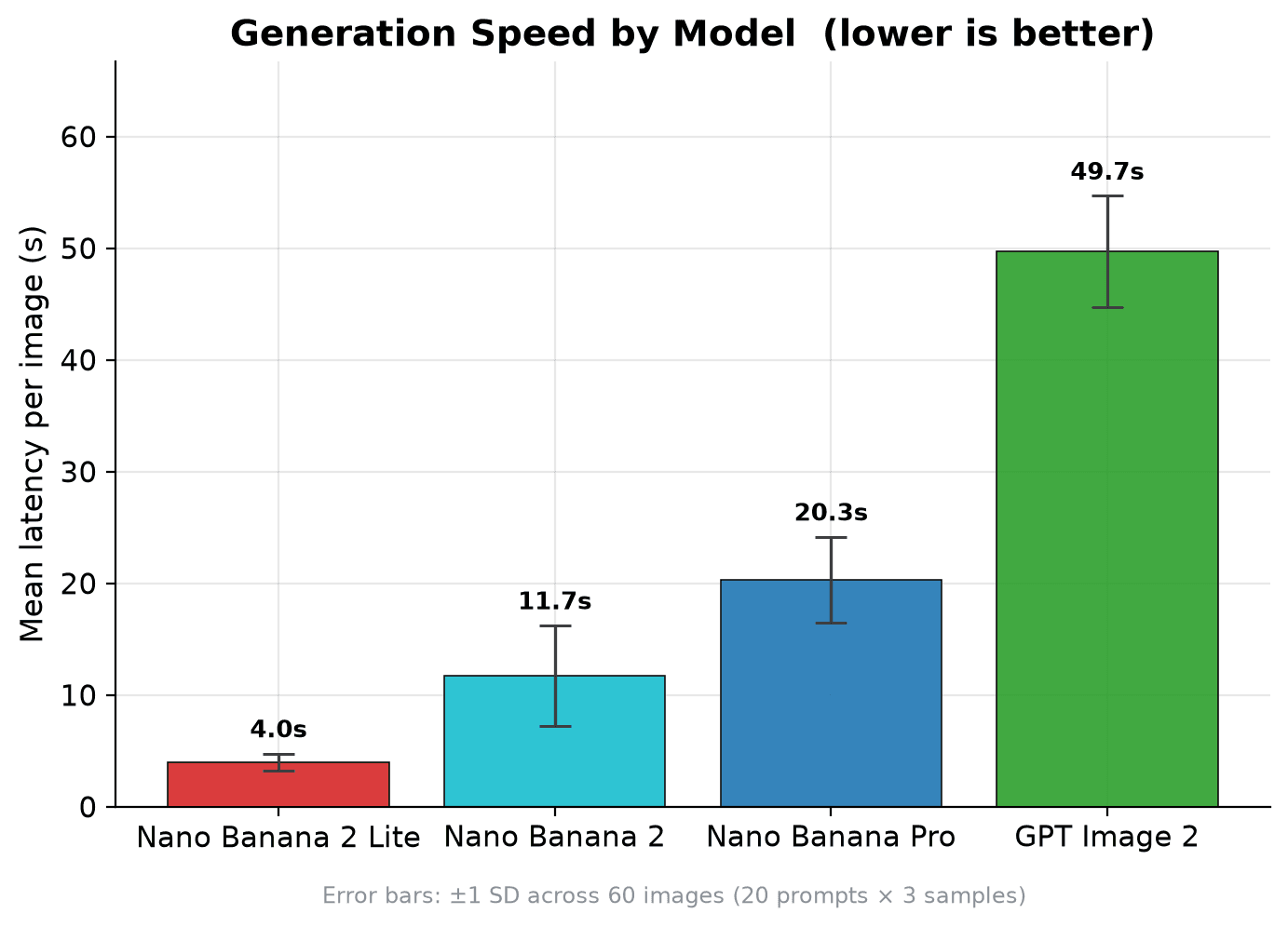
Latency is the cleanest result in the study. Nano Banana 2 Lite was the fastest model by a wide margin, with a mean latency of 4.0 seconds, median latency of 3.8 seconds, and p95 latency of 5.5 seconds. Nano Banana 2 was next at 11.1 seconds median, followed by Nano Banana Pro at 19.2 seconds and GPT Image 2 at 49.0 seconds.
That difference matters because scientific figure generation is almost never a one-shot call. A researcher adjusts labels, fixes an axis, tries a cleaner layout, changes a color, or asks the agent to make the diagram match the surrounding text. In an agent run, image generation is also just one step among many. A 50-second image call stalls the whole chain, while a sub-5-second call keeps the loop responsive.
 Figure 2. Generation latency.
 Nano Banana 2 Lite returns images in about four seconds on average, while GPT Image 2 is close to 50 seconds.
 Figure 3. Latency distribution. The box plot shows that
 Nano Banana 2 Lite is not just fast on average. Its spread is also tight, with p95 latency near 5.5 seconds.
The report's arithmetic makes the practical point. A figure-rich analysis with 30 visuals and about three iterations per visual is roughly 90 generations. At Nano Banana 2 Lite latency, that is about six minutes of generation time. At GPT Image 2 latency, the same session is about 73 minutes. That is the difference between keeping figure generation inside a live research conversation and pushing it into an overnight or background step.
Where Fast Generation Matters
Fast scientific image generation is most valuable when the figure is part of an active reasoning loop rather than a final artifact. A scientific agent may need to sketch a proposed experimental design, visualize a mechanism, compare alternative hypotheses, or explain an analysis step while it is still deciding what to do next. In those cases, the image is a thinking surface. If it takes almost a minute to appear, the agent and the researcher lose momentum.
One important use case is autonomous report writing. K-Dense agents often assemble dense technical reports with many diagrams, pathway sketches, workflow schematics, assay layouts, and explanatory figures. A fast model lets the agent draft the full visual spine of the report, then reserve slower high-quality generation for the few figures that need final polish.
Another use case is interactive scientific tutoring and review. When a researcher asks why a model chose a docking pose, how a circuit is wired, what a biological pathway implies, or where a thermodynamic cycle went wrong, the agent can answer with a quick visual rather than only text. The value is not that every quick diagram is publication-ready. The value is that the visual arrives while the question is still live.
Fast generation also matters for experimental planning and protocol design. An agent can rapidly mock up plate layouts, microscopy workflows, sample-preparation steps, instrument configurations, or branching decision trees. Those visuals help humans catch mistakes early, especially when the alternative is parsing a long textual protocol.
Finally, speed matters in large agent runs where image generation is one tool call among many. A drug-discovery agent might generate molecule-series summaries, target diagrams, assay cartoons, and report graphics in the same run. A materials-science agent might sketch crystal structures, phase diagrams, and processing workflows. A climate or aerospace agent might produce many explanatory schematics while comparing scenarios. In all of these cases, a fast image model keeps visualization inside the agent loop instead of turning it into the bottleneck.
Quality Still Belongs to GPT Image 2
Raw quality tells a different story from latency. GPT Image 2 led the benchmark with a composite score of 8.64 out of 10. Nano Banana Pro and Nano Banana 2 were nearly tied at 7.60 and 7.59. Nano Banana 2 Lite scored 6.70, which is useful for fast iteration but clearly behind the highest-quality model on scientific correctness, text, prompt adherence, and clarity.
That gap is visible in the dimension breakdown. GPT Image 2 scored 7.33 on scientific accuracy, 9.58 on text legibility, 9.55 on prompt adherence, 8.38 on visual clarity, and 8.75 on aesthetics. Nano Banana 2 Lite scored 5.23, 7.30, 7.72, 6.63, and 7.68 on the same dimensions.
 Figure 4. Composite quality. GPT Image 2 has the strongest raw figure quality, while
 Nano Banana 2 Lite trails the field on composite score.
 Figure 5. Rubric dimensions. Scientific accuracy is the lowest-scoring dimension for every model, which is exactly why scientific figures are a hard test.
The most important quality result is not only which model wins. It is that every model struggles most with the science itself. Text rendering has improved substantially across modern image models, and many labels are now legible. But scientific accuracy still lags because the model has to preserve structure, relationships, notation, scale, and domain conventions at the same time.
 Figure 6. Quality profile. GPT Image 2 encloses the other models across the rubric, while
 Nano Banana 2 Lite is most competitive on aesthetics and prompt adherence.
 Figure 7. Score distribution. The spread matters because a model that occasionally reaches high scores can still be risky if its lower tail contains plausible-looking scientific errors.
The Overall Score Is a Product Choice
The benchmark uses a transparent combined score because K-Dense has to choose defaults for real workflows, not abstract winners. The formula is simple: quality equals the composite score times 10, speed equals 100 times the fastest median latency divided by the model's median latency, and overall equals 70 percent quality plus 30 percent speed.
Under that 70/30 weighting, Nano Banana 2 Lite wins with an overall score of 76.9. Nano Banana 2 ranks second at 63.3, GPT Image 2 ranks third at 62.8, and Nano Banana Pro ranks fourth at 59.1. The ranking is sensitive to weighting, and it should be. If the product goal is final publication-quality figures, raw quality should dominate. If the product goal is fast iteration inside an autonomous research agent, latency deserves real weight.
| Rank | Model | Overall | Quality | Speed | Composite | Median Latency |
|---|---|---|---|---|---|---|
| 1 | Nano Banana 2 Lite |
76.9 | 67.0 | 100.0 | 6.70 | 3.8 s |
| 2 | Nano Banana 2 | 63.3 | 75.9 | 34.0 | 7.59 | 11.1 s |
| 3 | GPT Image 2 | 62.8 | 86.4 | 7.7 | 8.64 | 49.0 s |
| 4 | Nano Banana Pro | 59.1 | 76.0 | 19.6 | 7.60 | 19.2 s |
 Figure 8. Speed-quality frontier. The ideal point is top-left: high quality and low latency. GPT Image 2 is highest, but
 Nano Banana 2 Lite sits farthest left.
This is the honest conclusion: there is no single universal winner. There is a frontier. GPT Image 2 is the quality-first choice. Nano Banana 2 Lite is the interaction-first choice. Nano Banana 2 is a middle point with respectable quality and much better latency than GPT Image 2. Which model is best depends on how much waiting a researcher or agent workflow can tolerate.
Strength Varies by Scientific Field
The discipline heatmap is a useful reminder that a single aggregate score can hide important differences. GPT Image 2 stayed strong across most fields and peaked in physical chemistry, physics, and thermal engineering. Nano Banana 2 did especially well in electrical engineering and neuroscience. Nano Banana 2 Lite was relatively stronger in astronomy and physics, but weaker in biology, thermal engineering, electrical engineering, and aerospace.
Some of this variation is about visual form. Physics and astronomy prompts often have cleaner geometric structure and fewer dense biological labels. Biology and engineering diagrams often require many small components with leader lines, text, and exact topology. Those are precisely the cases where a model can make an image that looks plausible but fails the scientific purpose.
 Figure 9. Discipline heatmap. Each cell has only 3 to 6 images, so this should be read as directional rather than definitive. Still, it shows that field-level behavior is not uniform.
For product use, this points toward routing rather than a single hard-coded default forever. Fast models can power drafts, exploration, and repeated agent calls. Higher-quality models can be used for finalization, dense label-heavy figures, or domains where the current fast model is weakest. The right product behavior is not merely "pick the winner." It is "pick the right model for the figure's job."
Comparison Atlas: One Prompt, Four Models
The aggregate charts tell the benchmark story, but the model differences are easiest to understand prompt by prompt. The atlas below shows one representative generation for every prompt in the benchmark, using sample 1 from each model. Each card is open by default so the full comparison is visible, and it can be collapsed while reviewing the post.
1. bio-cell (Biology)
Prompt: A clean, professionally labeled scientific cross-section diagram of a eukaryotic animal cell, drawn in a biology-textbook illustration style on a white background. Clearly show and label, with thin leader lines and legible sans-serif text, the following organelles: nucleus, nucleolus, nuclear envelope, rough endoplasmic reticulum, smooth endoplasmic reticulum, Golgi apparatus, mitochondria, lysosome, ribosomes, centrioles, cytoskeleton, cytoplasm, and plasma membrane. Add a bold title at the top reading 'Eukaryotic Animal Cell'.


2. bio-central-dogma (Molecular Biology)
Prompt: An educational molecular-biology infographic illustrating the central dogma, flowing left to right: a DNA double helix, transcription producing mRNA, and translation producing a protein. Depict and label RNA polymerase on the DNA, the mRNA strand exiting the nucleus, a ribosome reading codons, tRNA molecules carrying amino acids, and the growing polypeptide chain. Annotate the two stages with the text 'Transcription (nucleus)' and 'Translation (cytoplasm)', and give the figure the title 'The Central Dogma of Molecular Biology'.


3. bio-enzyme-kinetics (Biochemistry)
Prompt: A precise scientific graph of Michaelis-Menten enzyme kinetics, plotting the reaction initial velocity V0 (y-axis) against substrate concentration [S] (x-axis). Draw the characteristic hyperbolic saturation curve approaching a horizontal asymptote, and clearly label the maximum velocity Vmax as a dashed horizontal asymptote, the half-maximal velocity Vmax/2, and the Michaelis constant Km marked on the x-axis at the substrate concentration where velocity equals Vmax/2. Include the Michaelis-Menten equation as text 'V0 = (Vmax * [S]) / (Km + [S])', add axis titles with units, gridlines, and the title 'Michaelis-Menten Enzyme Kinetics'.


4. neuro-action-potential (Neuroscience)
Prompt: A precise scientific line graph of a neuronal action potential plotting membrane potential in millivolts (y-axis, from -90 to +50 mV) against time in milliseconds (x-axis). Label the resting potential at -70 mV, the threshold at -55 mV, the rapid depolarization, the peak at +40 mV, repolarization, the hyperpolarization undershoot, and the return to rest. Annotate the phases with 'Na+ channels open' and 'K+ channels open', include gridlines and axis titles, and title the plot 'Action Potential'.


5. chem-sn2 (Chemistry)
Prompt: A clean organic-chemistry reaction-mechanism diagram of an SN2 nucleophilic substitution on a white background. Show the nucleophile (hydroxide, OH-) attacking a primary alkyl halide from the side opposite the leaving group (bromide, Br-), the trigonal-bipyramidal transition state drawn in square brackets with partial bonds, and the product with inverted stereochemistry. Use curved arrows for electron flow and add text labels 'Nucleophile', 'Transition state', 'Leaving group', and 'Backside attack - inversion of configuration'. Title it 'SN2 Reaction Mechanism'.


6. chem-energy-profile (Physical Chemistry)
Prompt: A scientific potential-energy diagram plotting potential energy (y-axis) against reaction coordinate (x-axis) for an exothermic reaction, comparing an uncatalyzed pathway and a catalyzed pathway as two labeled curves. Mark and label the reactants, the products, the transition state at each peak, the activation energy Ea for both pathways (showing the catalyzed Ea is lower), and the overall enthalpy change delta-H drawn as a negative drop. Include axis titles and the title 'Reaction Energy Profile: Catalyzed vs. Uncatalyzed'.


7. chem-titration (Chemistry)
Prompt: A scientific titration curve plotting pH (y-axis, 0 to 14) against volume of titrant added in mL (x-axis) for a strong acid titrated with a strong base. Show the characteristic S-shaped curve, and clearly label the initial acidic pH, the steep equivalence point at pH 7, and the leveling-off in the basic region. Add a dashed line marking the equivalence point and annotate it, include gridlines and axis titles, and give it the title 'Strong Acid - Strong Base Titration Curve'.


8. phys-projectile (Physics)
Prompt: A physics diagram of projectile motion on a white background showing a smooth parabolic trajectory of a launched ball. Draw the initial velocity vector v0 at launch angle theta above the horizontal, decomposed into its horizontal component v0*cos(theta) and vertical component v0*sin(theta), the downward gravitational acceleration g, the maximum height H at the apex, and the total horizontal range R. Include the kinematic equations for range and maximum height as text, label all vectors and quantities, and title the figure 'Projectile Motion'.


9. phys-double-slit (Physics)
Prompt: A clean optics schematic of Young's double-slit interference experiment, viewed from above. Show a coherent monochromatic light source, a barrier with two narrow slits separated by distance d, light waves diffracting and overlapping, and the resulting pattern of alternating bright and dark fringes on a screen a distance L away. Label the slit separation d, the screen distance L, the path difference d*sin(theta), and the fringe-spacing relation, and add the title 'Young's Double-Slit Interference'.


10. ee-opamp (Electrical Engineering)
Prompt: A clean electronic schematic of a non-inverting operational-amplifier circuit drawn with standard circuit symbols on a white background. Show the op-amp triangle symbol with + and - inputs and an output, the input signal Vin connected to the non-inverting input, a feedback resistor Rf from the output to the inverting input, a resistor R1 from the inverting input to ground, and the output node labeled Vout. Add the gain equation as text: 'Vout / Vin = 1 + Rf / R1', and title the schematic 'Non-Inverting Amplifier'.


11. mech-stress-strain (Mechanical Engineering)
Prompt: An annotated engineering stress-strain curve for a ductile metal, plotting engineering stress in MPa (y-axis) against strain (x-axis, dimensionless). Clearly label the linear elastic region, the proportional limit, the yield strength, the ultimate tensile strength at the peak, the necking region, and the fracture point. Indicate Young's modulus E as the slope of the elastic region with a small triangle, include axis titles, and give the figure the title 'Stress-Strain Curve of a Ductile Metal'.


12. mech-four-stroke (Mechanical Engineering)
Prompt: A technical illustration of the four-stroke internal-combustion engine cycle shown as four side-by-side cylinder cross-sections. In each panel draw the piston, connecting rod, crankshaft, intake valve, exhaust valve, and spark plug, with an arrow showing piston direction and the valve states. Caption the panels in order 'Intake', 'Compression', 'Power', and 'Exhaust', label the key components, and title the whole figure 'Four-Stroke Engine Cycle'.


13. mech-rankine (Thermal Engineering)
Prompt: A labeled thermodynamic schematic of a steam Rankine power cycle on a white background, with four components connected in a loop by piping with flow arrows: a boiler, a turbine, a condenser, and a feed pump. Mark the four state points 1, 2, 3, and 4 between components, and label the energy transfers: heat added Q_in at the boiler, work output W_turbine, heat rejected Q_out at the condenser, and pump work W_pump. Include a small inset temperature-entropy (T-s) diagram of the cycle, and title it 'Rankine Cycle'.


14. aero-airfoil (Aerospace)
Prompt: An aerodynamics diagram of an airfoil (wing cross-section) in a horizontal airflow, on a white background. Draw curved streamlines flowing over and under the airfoil, the chord line, the relative wind, and the angle of attack alpha between them. Show the four forces of flight as labeled vectors: lift (up), weight (down), thrust (forward), and drag (backward). Include the lift equation as text 'L = 0.5 * rho * v^2 * S * C_L', label all elements, and title the figure 'Airfoil Aerodynamics and the Four Forces of Flight'.


15. aero-hohmann (Aerospace)
Prompt: A clean orbital-mechanics diagram on a dark space background showing a Hohmann transfer between two coplanar circular orbits around a central planet. Draw the inner circular orbit of radius r1, the outer circular orbit of radius r2, and the elliptical transfer orbit tangent to both. Mark the first burn delta-v1 where the spacecraft leaves the inner orbit (periapsis of the transfer) and the second burn delta-v2 where it circularizes at the outer orbit (apoapsis), with arrows for direction of motion. Label the orbits, radii, and burns, and title it 'Hohmann Transfer Orbit'.


16. astro-hr-diagram (Astronomy)
Prompt: A scientific Hertzsprung-Russell diagram plotting stellar luminosity relative to the Sun (y-axis, logarithmic from 0.0001 to 1,000,000) against surface temperature in Kelvin (x-axis, reversed so hot is on the left). Show and label the diagonal main sequence band, the red giants region, the supergiants region, and the white dwarfs region, mark the Sun's position with a dot, and place the spectral classes O, B, A, F, G, K, M along the top axis. Include axis titles and the title 'Hertzsprung-Russell Diagram'.


17. astro-star-lifecycle (Astronomy)
Prompt: An astronomy flow diagram on a dark cosmic background depicting the life cycle of a star, branching by mass. Start from a stellar nebula, then a protostar and the main sequence, then split into two labeled paths: a low-mass (Sun-like) path leading to red giant, then planetary nebula, then white dwarf; and a high-mass path leading to red supergiant, then supernova, then neutron star or black hole. Use arrows between stages and label every stage with text, and title the figure 'Life Cycle of a Star'.


18. astro-black-hole (Astrophysics)
Prompt: A high-fidelity astrophysical visualization of a black hole on a dark starfield background, with clear scientific labels and leader lines. Show and label the central singularity, the spherical event horizon, the glowing accretion disk of superheated matter spiraling inward, the photon sphere, and the relativistic jets emitted along the rotation axis. Indicate the Schwarzschild radius with a labeled arrow, and give the image the title 'Anatomy of a Black Hole'.


19. earth-plate-tectonics (Earth Science)
Prompt: A geology-textbook cross-section diagram illustrating the three types of plate-tectonic boundaries in one cutaway view of Earth's crust and upper mantle. Show and label a divergent boundary at a mid-ocean ridge with upwelling magma, a convergent boundary with oceanic-plate subduction forming an ocean trench and a volcanic arc, and a transform boundary with plates sliding past each other. Label the lithosphere, asthenosphere, mantle convection currents, and magma, and title the figure 'Plate Tectonic Boundaries'.


20. mat-crystal-phase (Materials Science)
Prompt: A two-panel scientific figure on a white background. Left panel: a labeled face-centered cubic (FCC) crystal unit cell showing atoms at the corners and face centers, with the lattice parameter 'a' indicated, titled 'FCC Unit Cell'. Right panel: a labeled pressure-temperature phase diagram of water, with axes pressure (y) and temperature (x), showing the solid, liquid, and vapor regions, the phase-boundary curves, the triple point, and the critical point clearly marked, titled 'Phase Diagram of Water'. Add an overall title 'Crystal Structure and Phase Diagram'.


Reading across the atlas, the pattern is consistent with the aggregate metrics. GPT Image 2 is usually the cleanest and most faithful on dense labels and equations. Nano Banana 2 Lite is often good enough for fast iteration, especially on simpler physical diagrams, but it needs review on label-heavy biology and engineering figures. The practical value is that reviewers can see both sides of the tradeoff instead of taking the leaderboard on faith.
What This Means for K-Dense
For K-Dense, the product implication is not that every figure should always use the fastest model. The implication is that speed belongs in the model-selection policy. Scientific agents create drafts, intermediate artifacts, report figures, explainer diagrams, and final visuals. Those are different jobs, and they should not all pay the same latency tax.
The fastest model is especially valuable for intermediate steps. When an agent needs to sketch an experimental setup, create a quick explanatory diagram, or iterate on report visuals during a long run, waiting 50 seconds per image can dominate the runtime. At four seconds, image generation can become a normal part of the agent loop.
The highest-quality model remains valuable for finalization. GPT Image 2's quality lead is real, especially for scientific accuracy and dense labels. A practical workflow can use Nano Banana 2 Lite for rapid drafts and GPT Image 2 for final pass generation when the figure is headed into a user-facing deliverable. The benchmark gives us the data to make that tradeoff explicitly.
Limitations
This is a benchmark of 20 prompts, not a complete map of scientific visualization. The prompts span biology, chemistry, physics, engineering, earth science, astronomy, and materials science, but they do not cover every diagram type a researcher might request. The discipline heatmap is especially small, with only 3 to 6 images per cell, so field-level conclusions should be treated as directional.
The scoring used a single LLM vision judge, Claude Opus 4.8, at temperature 0. That makes the process consistent and scalable, but it is not the same as a human expert panel. A future version should add human review for a subset of figures, especially for subtle scientific accuracy failures.
The overall score is deliberately subjective. We chose 70 percent quality and 30 percent speed because K-Dense cares about both final output and interactive agent performance. A publication-only benchmark would weight quality more heavily and rank GPT Image 2 first. A real-time drafting benchmark might weight speed even more heavily and widen Nano Banana 2 Lite's lead.
The benchmark also used fixed generation settings and fixed model versions at one point in time. Actual output dimensions differed by provider: GPT Image 2 returned 1536x1024 images, the two Nano Banana models returned 1376x768 images, and Nano Banana 2 Lite returned 1408x768 images. Nano Banana 2 Lite is unreleased and still changing, and the other providers will also improve. These numbers should be read as a snapshot of the tested systems, not a permanent ranking of image generation.
Finally, the benchmark measured latency and quality, but did not publish a dollar-denominated cost comparison. In practice, cost and latency compound together across repeated generations, especially in agent sessions that produce many figures. The qualitative product conclusion is still clear, but a full economic benchmark should include provider pricing once the unreleased model has public pricing.
Conclusion
The benchmark gives us a useful and grounded answer. Nano Banana 2 Lite is not the best raw scientific image model in this study. GPT Image 2 is. But Nano Banana 2 Lite is fast enough to change how scientific figure generation feels inside a research product: 3.8 seconds median instead of 49.0 seconds, with all 60 generations completing successfully.
That speed matters because AI co-scientists do not generate one image in isolation. They iterate. They revise. They run tool chains. They produce reports full of diagrams, plots, and schematics. In that setting, the best model is not always the model with the highest single-image score. It is the model that gives the right quality at the right latency for the job.
For now, the practical policy is straightforward. Use GPT Image 2 when raw scientific figure quality matters most. Use Nano Banana 2 Lite when interaction speed, iteration volume, and agent responsiveness matter most. Then keep benchmarking, because the frontier is moving quickly and scientific accuracy remains the hardest part of the problem.
Related Reading
For the broader argument behind scientific agents, start with Introducing Scientific Agents and The Model Is No Longer the Bottleneck. They explain why the hard part of AI for science is increasingly the workflow around the model: verification, tools, context, and domain execution.
For adjacent benchmark work, see our studies on NVIDIA BioNeMo NIM skills, the pyOpenMS mass spectrometry skill, and the Rowan chemistry skill. Those posts ask a similar question in tool use rather than image generation: when does packaging scientific capability for agents change reliability, cost, and speed?
For product context, K-Dense Web vs. Scientific Agent Skills explains how hosted agents and open skills fit together, while Reproduction, Not Generation, Is the Future of AI for Science lays out why scientific AI systems need artifacts that can be checked, rerun, and improved.